18 Dec 2025
- Attendees:
Petrovic, D. McDonagh, D. Waterman, E. Krissinel
Results
Created this website to document progress.
Tried to process data from the original paper ([Clabbers et al., 2019]). There is a problem with rotation data (missing starting angle and oscillation). Problem with reading CBF header.
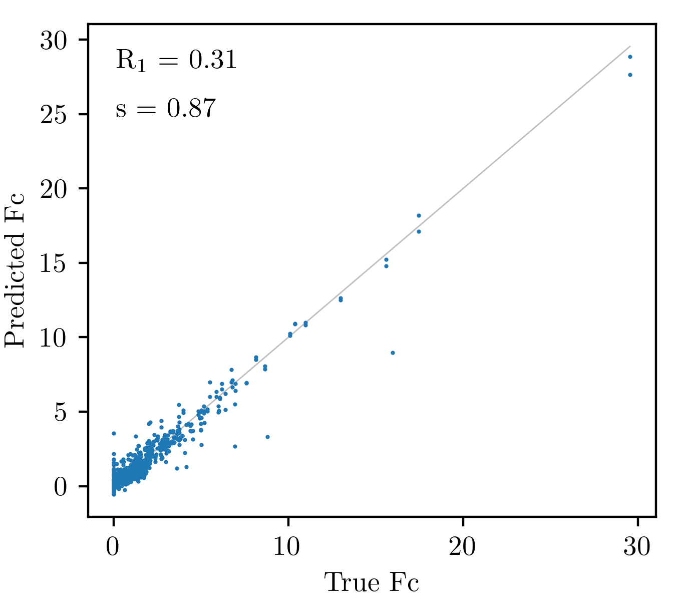
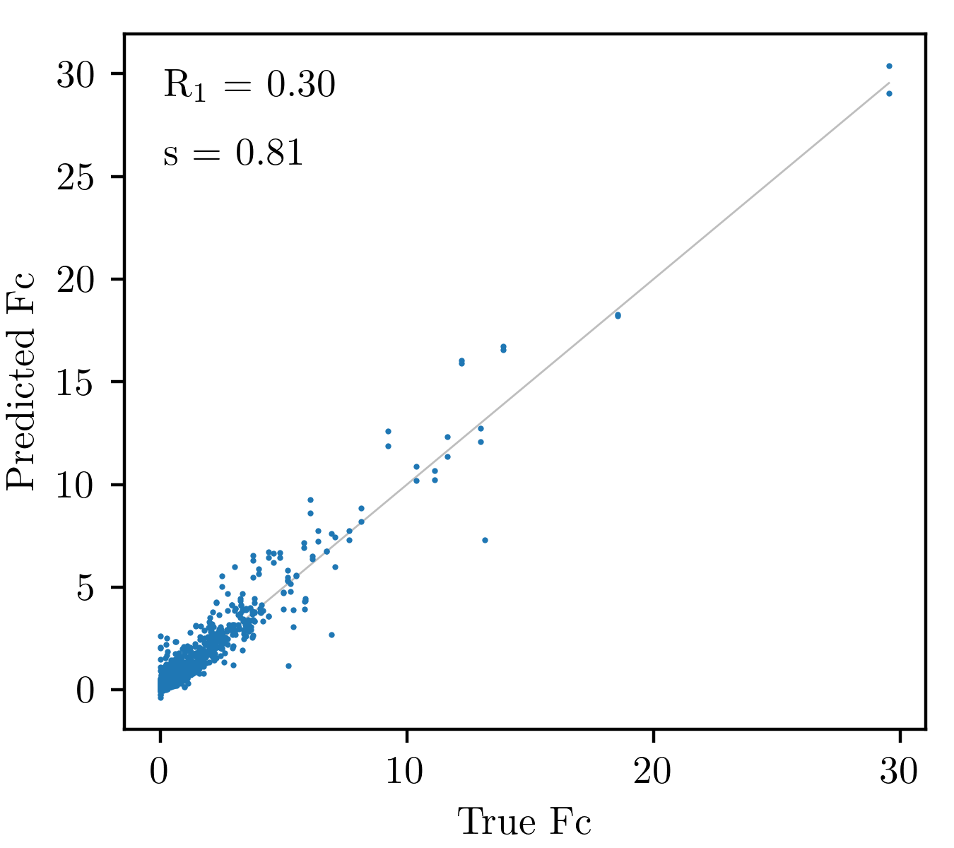
Created a global fitter function. Model built using these parameters:
Spot property: H, K, L, intensity, sigma, resolution
Dataset property: average \({\rm F}_o\), median \({\rm Fo}\)
|
|
|
Global prediction on training dataset. |
Global prediction on new dataset |
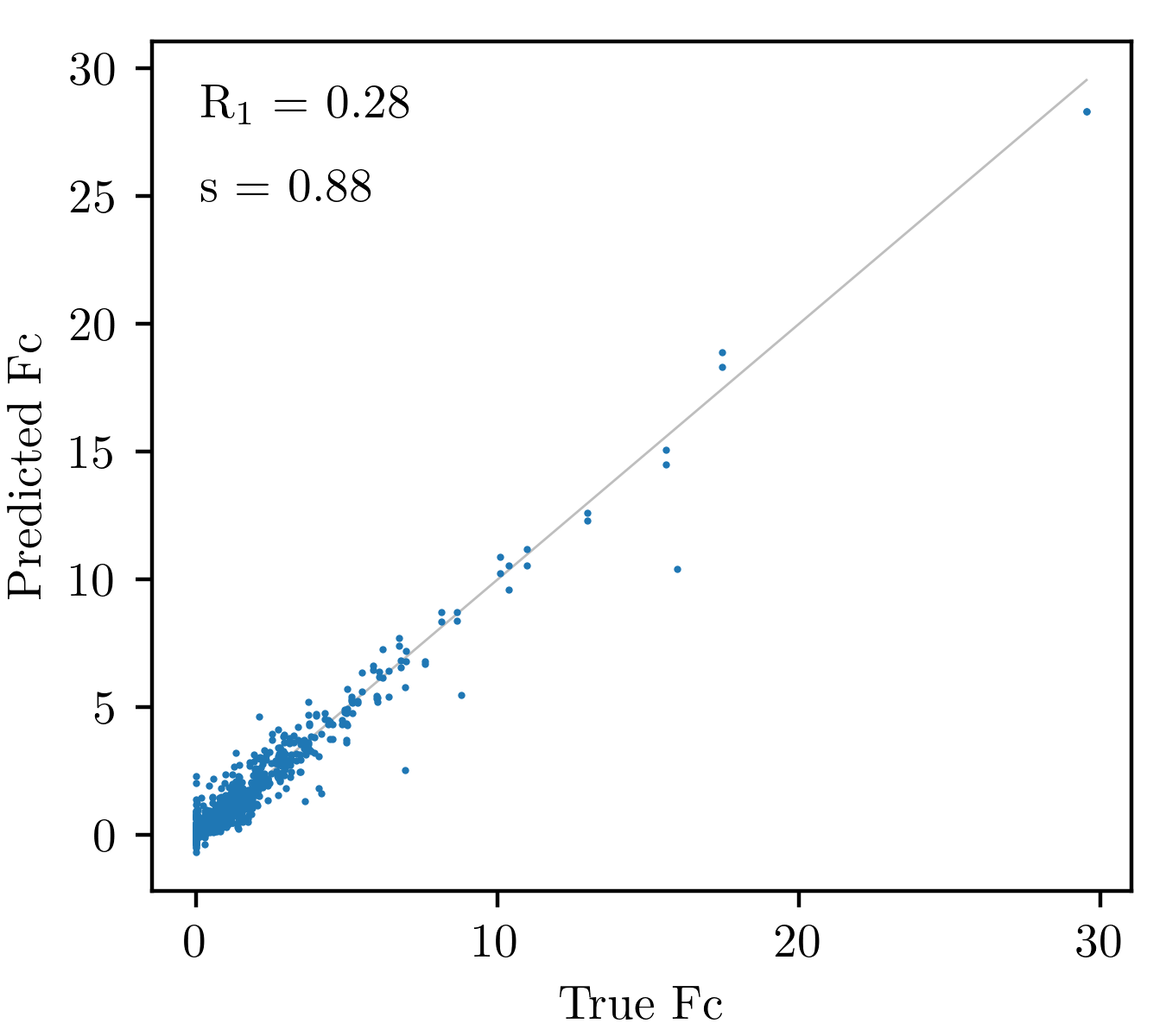
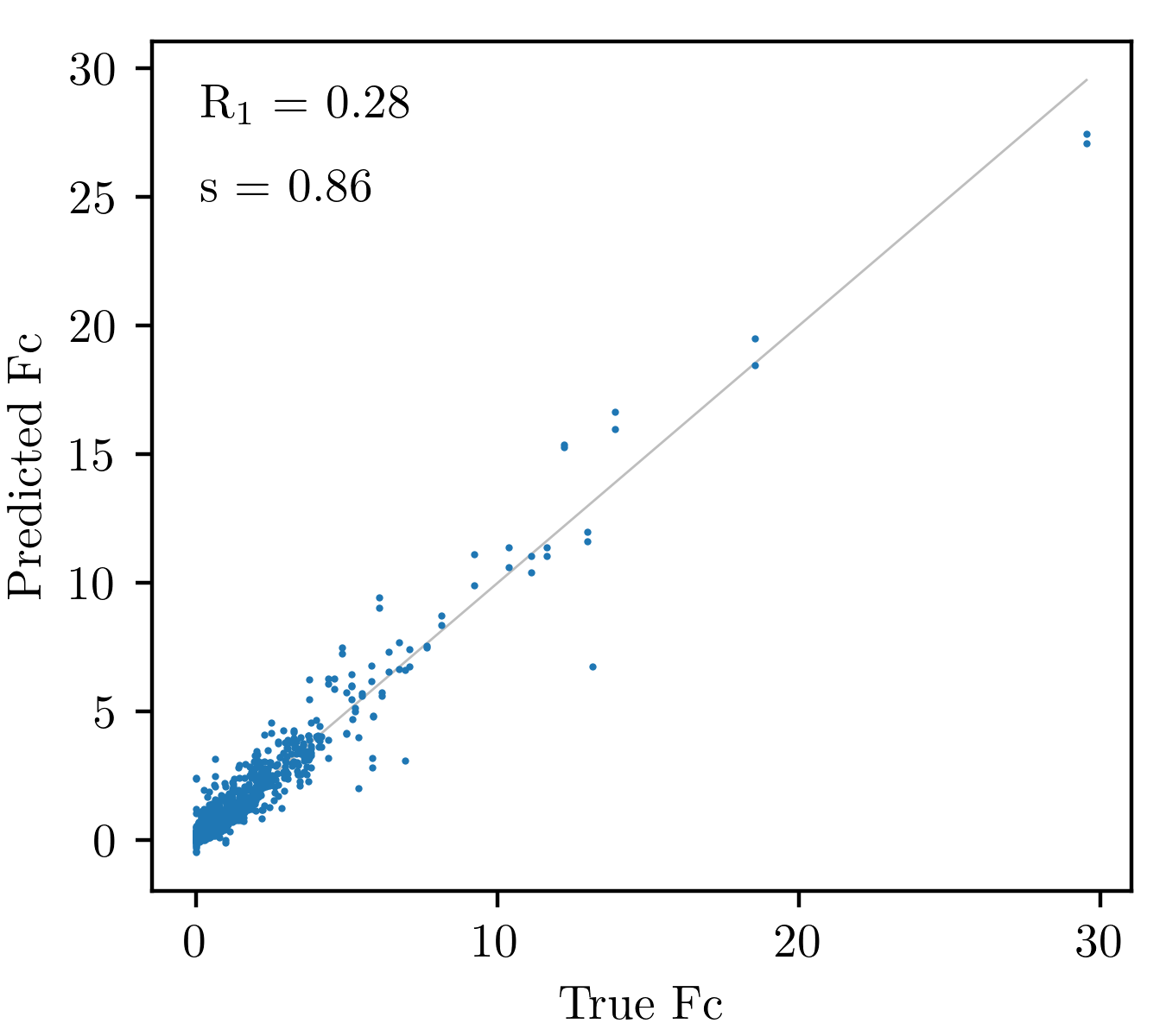
Created a local fitter function. Model built using these parameters
Spot property: H, K, L, intensity, sigma, resolution
Dataset property: average \({\rm F}_o\), median \({\rm Fo}\)
Neighbor property: min neighbor intensity, max neighbor intensity, 90 percentile neighbor intensity, IQR neighbor intensity, max neighbor resolution, min neighbor resolution, average neighbor resolution, number of neighbors, average neighbor intensity,
Neighbors are computed in real space (pixel distance).
|
|
|
Local prediction on training dataset. |
Local prediction on new dataset |
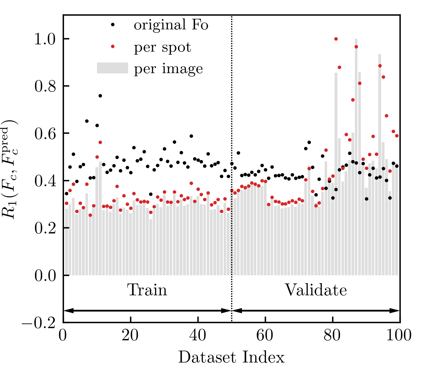
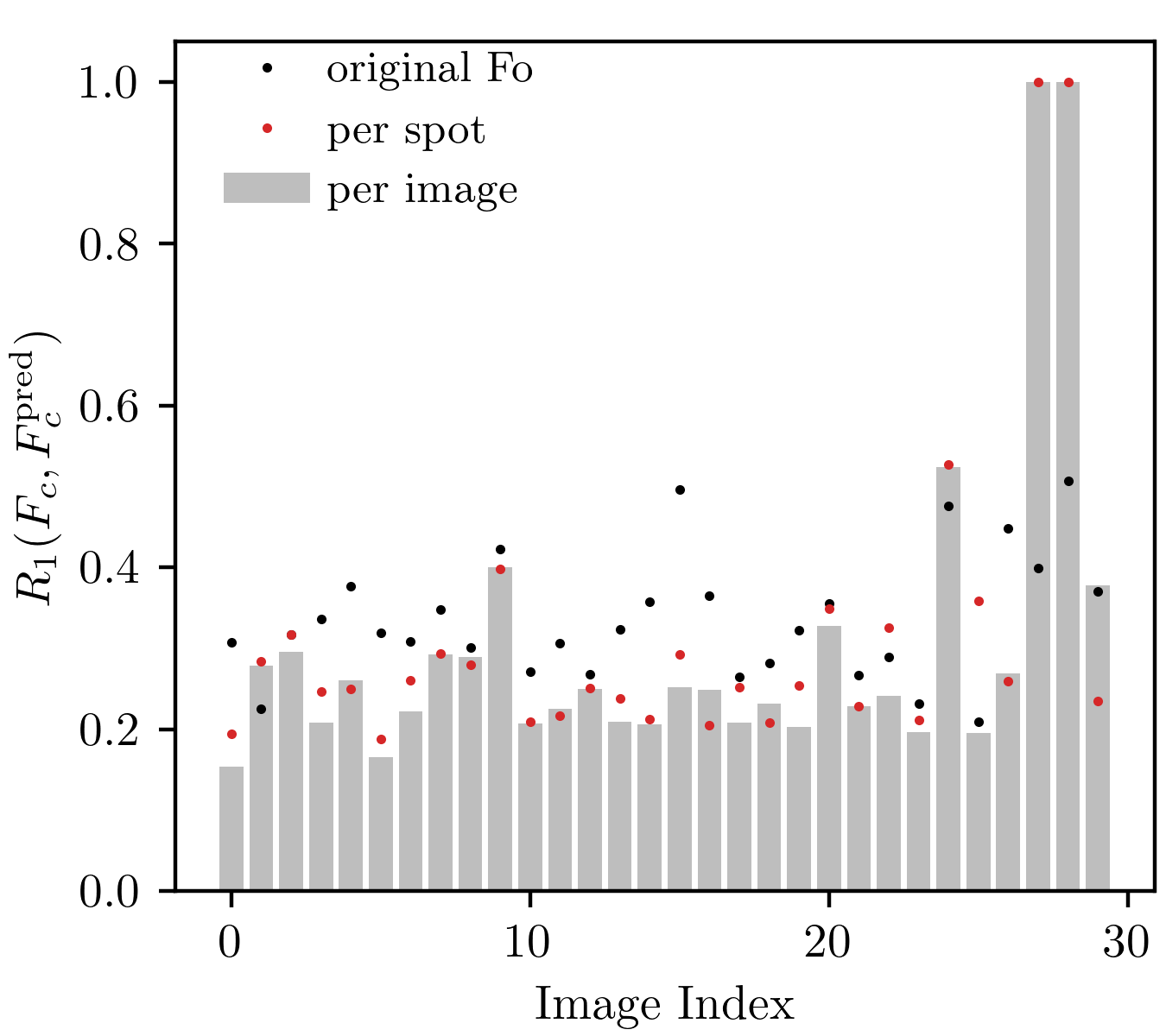
Comparing R1 factors (per image and for the whole dataset).
|
|
|
\(R_1\) across datasets. |
\(R_1\) per image. |
Discussion
In addition to \(R_1\), use maximum likelihood and entropy to assess the fit quality.
The GBT model should use spot coordinates in the inverse space (i.e. \(k_x\), \(k_y\), \(k_z\)) instead of Miller indices.
Use excitation error as a spot property.
Use distance on the Ewald sphere (instead of the real/detector space) to determine nearest neighbors of a spot.
Another approach might be to train CNNs on images of spots on the Ewald sphere.
Vary the GBT model size to get a better fit.