12 Mar 2026
- Attendees:
Petrovic, D. Waterman, D. McDonagh
Results
Explored possible ways abTEM simulation can be improved to better match measured data.
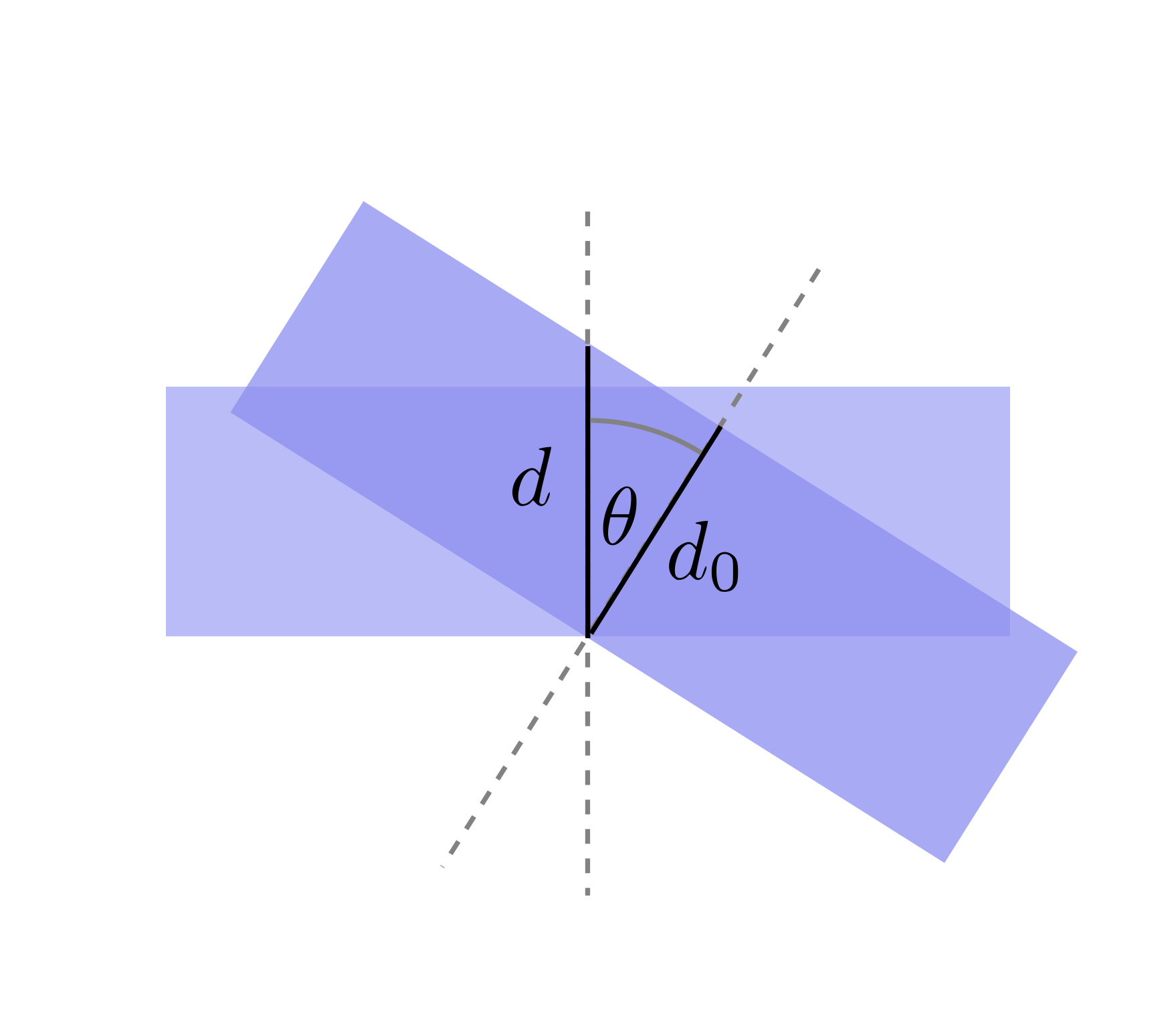
The sample thickness will change through the rotational scan depending on the sample geometry. For example, for an infinite slab with a single beam passing through (Fig. 1), the thickness correction is given by \(d(\theta) = d_0 / \cos(\theta)\), where \(d_0\) is the thickness at angle zero (the beam normal to the slab). This is now implemented for Bloch wave simulation.
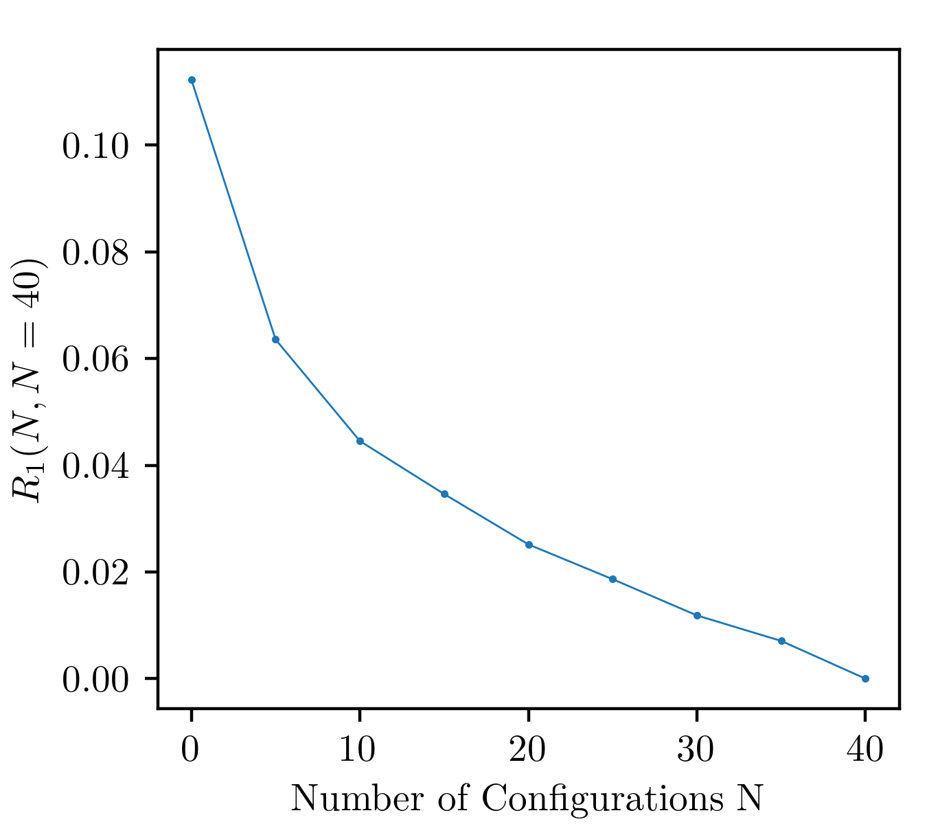
By default, abTEM performs simulations at zero temperature. The code allows simulation at a nonzero temperature, where the temperature is included by averaging over different lattice configurations. This is now implemented in our package (for Bloch waves), and we tested how results converge with the number of different configurations (Fig. 2). Although the graph in Fig. 2 does not clearly show convergence with the number of configurations, the computed \(R_1\) factor suggests that, neglecting temperature corrections, we are probably introducing an error of around 0-10%.
Another correction worth exploring in the future is the small-tilt-angle correction, or averaging across different thicknesses.
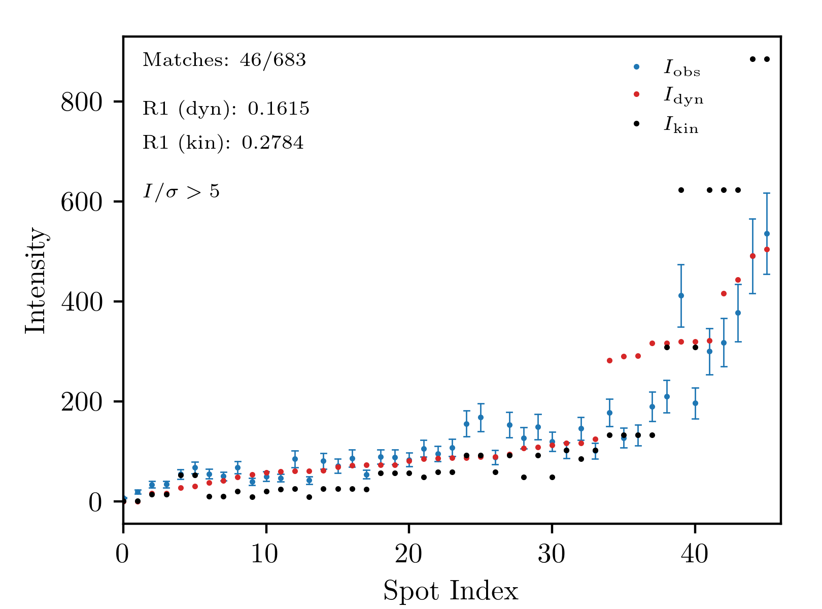
The resolution of the angle interpolation in abTEM also determines the accuracy of the integrated intensity. Thicker crystals require better resolution because the rocking curves become more jittery. For example, Fig. 6 from the 26th February meeting report was originally computed with 50 points interpolated over a one-degree angle. If we increase the angle resolution to 500 points per degree, the \(R_1\) factor for strong spots (\(I/\sigma > 5\)) drops to 0.16 for abTEM (Fig. 3). This is significantly lower than the value we obtain with the kinematic approximation (Gemmi).
|
|
|
Fig. 1: Change in thickness of an infinite slab as it rotates around a single pivot point at its bottom side. Note that different shapes will have different thicknesses depending on the rotation angle. |
Fig. 2: \(R_1\) factor scaling with the number of lattice configurations included in the abTEM Bloch wave simulation for non-zero temperature. The \(R_1\) factor is computed for a number of high-intensity spots (paracetamol at a single lattice orientation) from intensities obtained at a given number of temperature configurations, \(N\), compared to the maximum number of configurations used (\(N = 40\)). Results for zero configurations correspond to zero temperature. |
Fig. 3: Comparison between kinematic (Gemmi) and dynamic (abTEM) predictions of high-signal spots in paracetamol. The angle resolution used to compute the rocking curves with abTEM was \(1/500^{\circ}\), which resulted in further reduction of the \(R_1\) factor, as compared to the same result at the more crude resolution of \(1/50^{\circ}\) (Fig. 6 from Feb. 26th). Thickness correction from Fig. 1 was included in the simulation (the thickness at the zero angle was set to 166 nm). |
We tried our GBT model on the paracetamol data at two stages of processing: right after integration and at the final step (after scaling), when the data is usually exported to shelx. The results of processing with shelx are presented in the following table.
Paracetamol (\(1^{\circ}\) oscillation) |
All datasets (326) |
Excluding training (first 100 datasets) |
|---|---|---|
Original data |
\(R_1 = 0.246\) |
\(R_1 = 0.365\) |
GBT predicted (from integrated) |
\(R_1 = 0.190\) |
\(R_1 = 0.183\) |
GBT predicted (from scaled) |
\(R_1 = 0.220\) |
\(R_1 = 0.224\) |
Trying to extend the present model to other materials (Biotin in Fig. 4 and IRELOH in Fig. 5) shows its limitations. Instead of using Miller indices, we switched to spot positions in reciprocal space (\(k_x\), \(k_y\), \(k_z\)); however, this did not generalize our model. In both cases (biotin and IRELOH), applying our GBT model yields worse results than the original data, suggesting that the model’s learned functional form is not generalizable.
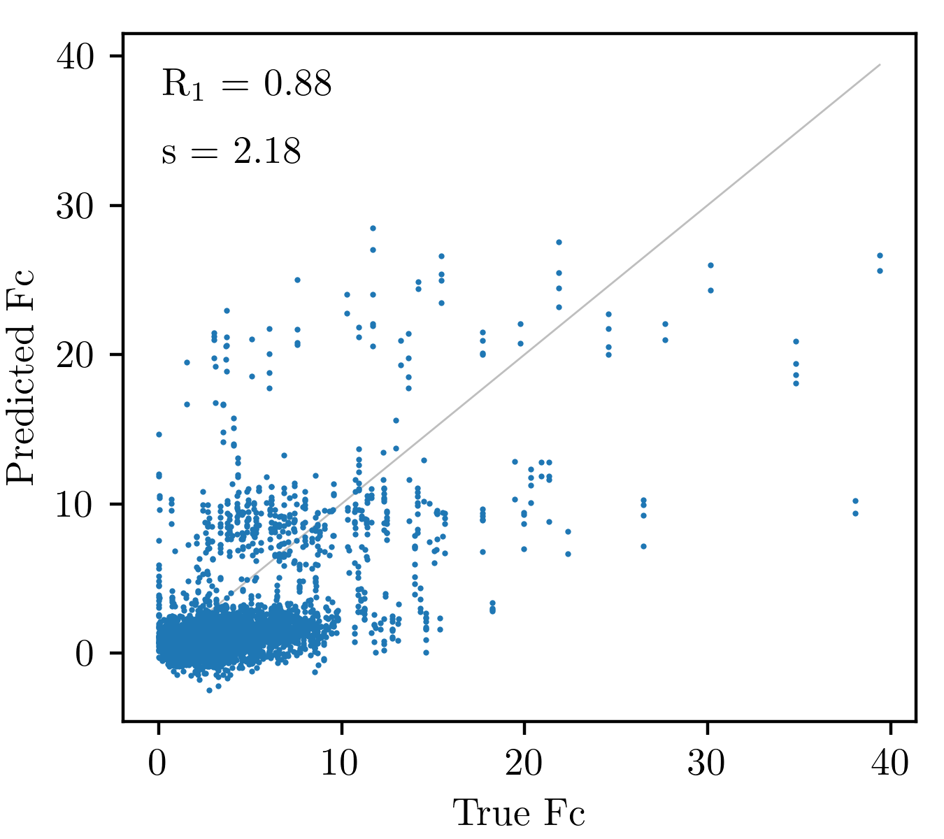
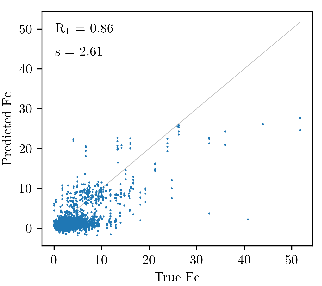
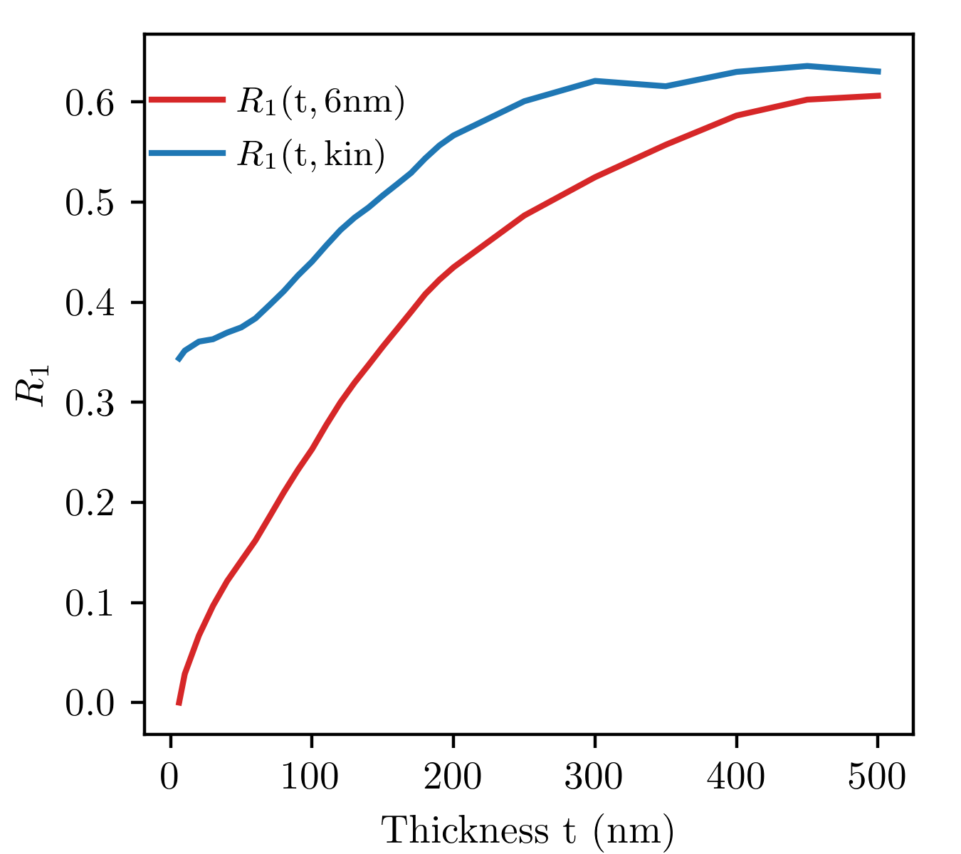
Fig. 4: Structure factors for Biotin (from DIALS tutorial), predicted using the GBT model trained on the first hundred datasets of paracetamol (1 degree).
Fig. 5: Structure factors for IRELOH, predicted using the GBT model trained on the first hundred datasets of paracetamol (1 degree).
Fig. 6: Scaling of the paracetamol spot intensities with the crystal thickness (no experimental data, only simulation). The \(R_1\) factor is computed between intensities obtained with Gemmi (no thickness) and abTEM for a given thickness (blue curve). Additionally, we compared how abTEM results scale with thickness (red curve), against the abTEM results at the minimal thickness (6 nm).
The last result (Fig. 6) shows how paracetamol data change with thickness. We compared simulated spot intensities (Bloch wave) from a single (one-degree) rotational scan with their kinematic prediction, with changing thickness (blue curve in Fig. 6). Similarly, we compared how Bloch wave results change with thickness (the reference point set to 6 nm) in the red curve. The conclusion is that spot intensities are highly thickness-dependent. This raises another question: can spots be grouped into those that are drastically affected by thickness and those that are not? d
Discussion
Check how Fig. 6 changes for zero thickness interpolation. Do kinematic and abTEM results converge to the same results when interpolated to zero thickness?
Run TPOT on your GBT model to further optimize it.
Apply changes to the GBT model to improve its generalizability to other materials. Change z-index to rotation angle, do not use excitation angle, use rotation angle difference instead. Do not use Miller indices; use \(k_x\), \(k_y\), and \(k_z\). Try with scaled intensities. Provide average intensity at the beam position.