19 Feb 2026
- Attendees:
Petrovic, D. Waterman, E. Krissinel
Results
Implemented a wrapper around the abTEM Bloch wave solver into Dynamic package. Now, it is possible to run both Bloch wave and Multislice simulations on the same unit-cell orientation and compare the results.
In the Multislice wrapper, the system can now be cut in three different ways: a sphere, a cuboid, or a cylinder (all aligned with the beam direction). The shape is “fixed in space,” whereas the crystal structure (unit cell) is free to rotate and follow the path taken from the actual measurements. In this way, the number of atoms in the computational volume will change from one orientation to another (as atoms drop in and out of the fixed shape). Fig. 1 shows a cross section for a crystal of paracetamol cut into a cylinder. We discovered that a cuboid might not be a good shape, because it introduces distortions along x and y directions (Fig. 2). However, this might be more an effect of a small cross-section of the sample, than the general property of the cuboid shape. It is possible that for larger samples, the effect disappears. For the cylinder shape, the distortion disappears (Fig. 3) due to rotational symmetry.
Fig. 4 shows the same diffraction image as Fig. 3, but now computed using Bloch waves. The high-intensity spots in both figures match the actual measurements, indicating that the unit cell orientation is correct.

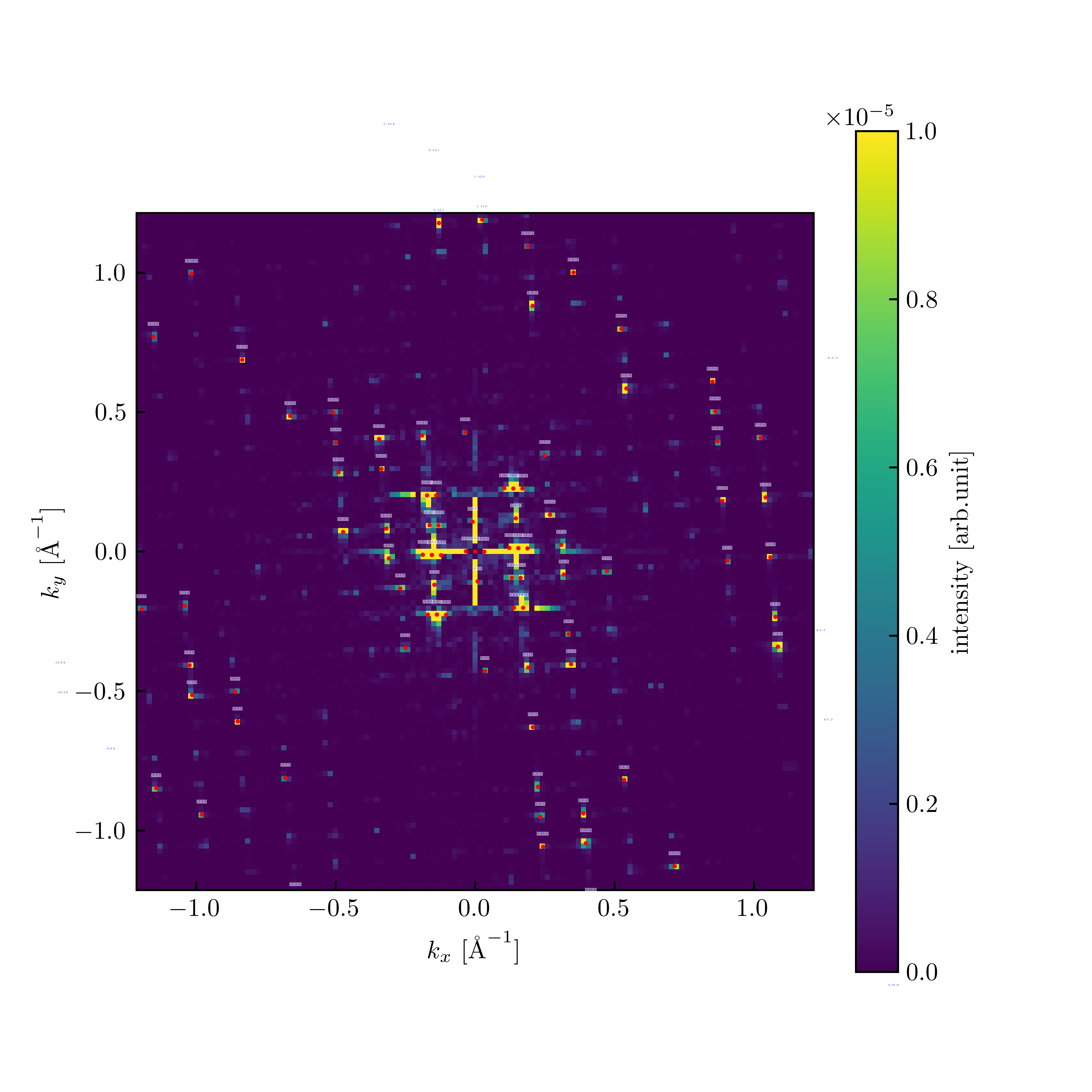
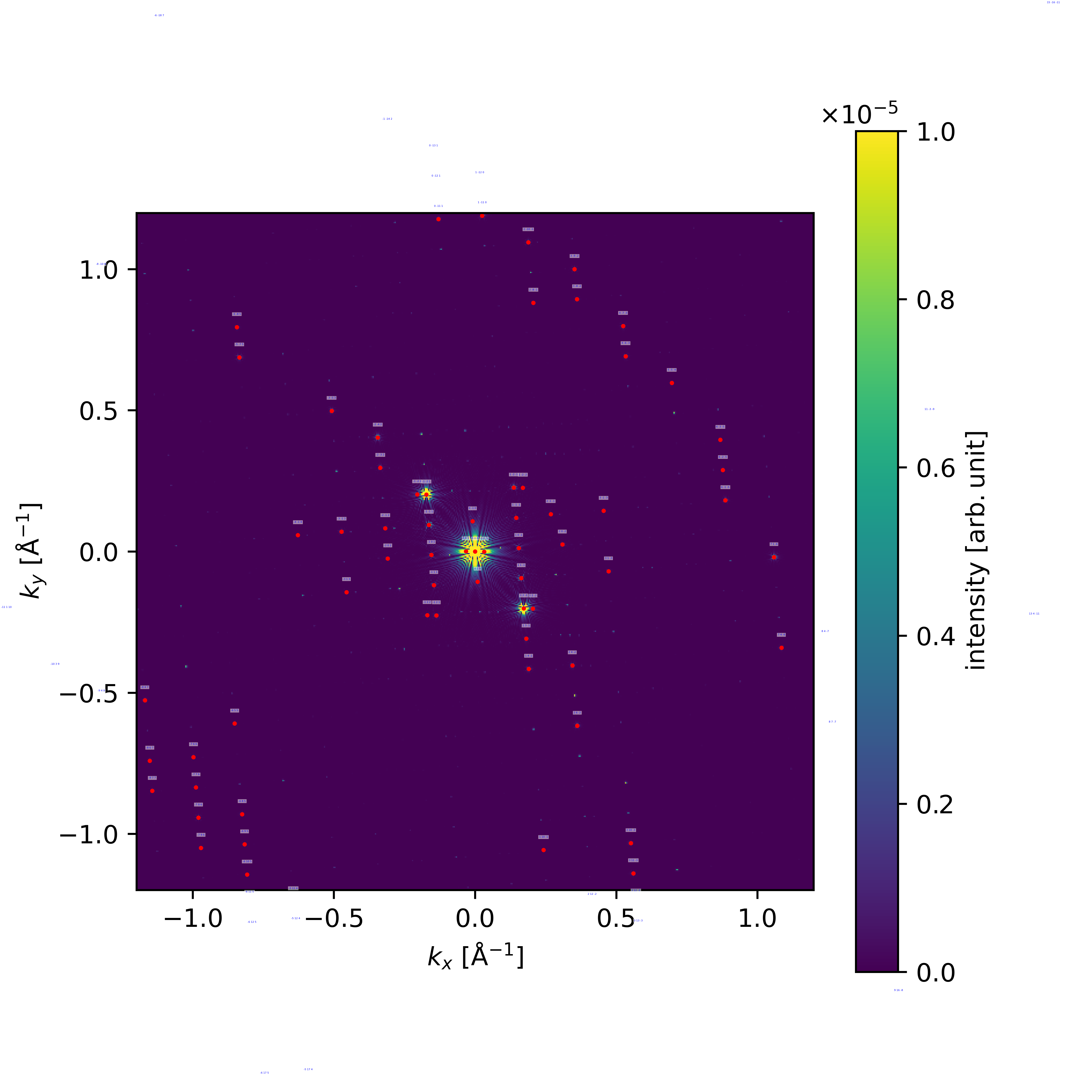
Fig. 1: A cross-section of a paracetamol crystal cut into a cylinder, created with abTEM.
Fig. 2: A diffraction pattern of the paracetamol crystal obtained for a cuboid shape. The actual orientation corresponds to one of the measured diffraction images.
Fig. 3: Same as Fig. 2, but now for a cylindrically cut crystal.
Once the error is corrected (i.e., the properly scaled intensities are read), the R1 in the GBT model drops significantly even before implementing any additional properties (Fig. 4).
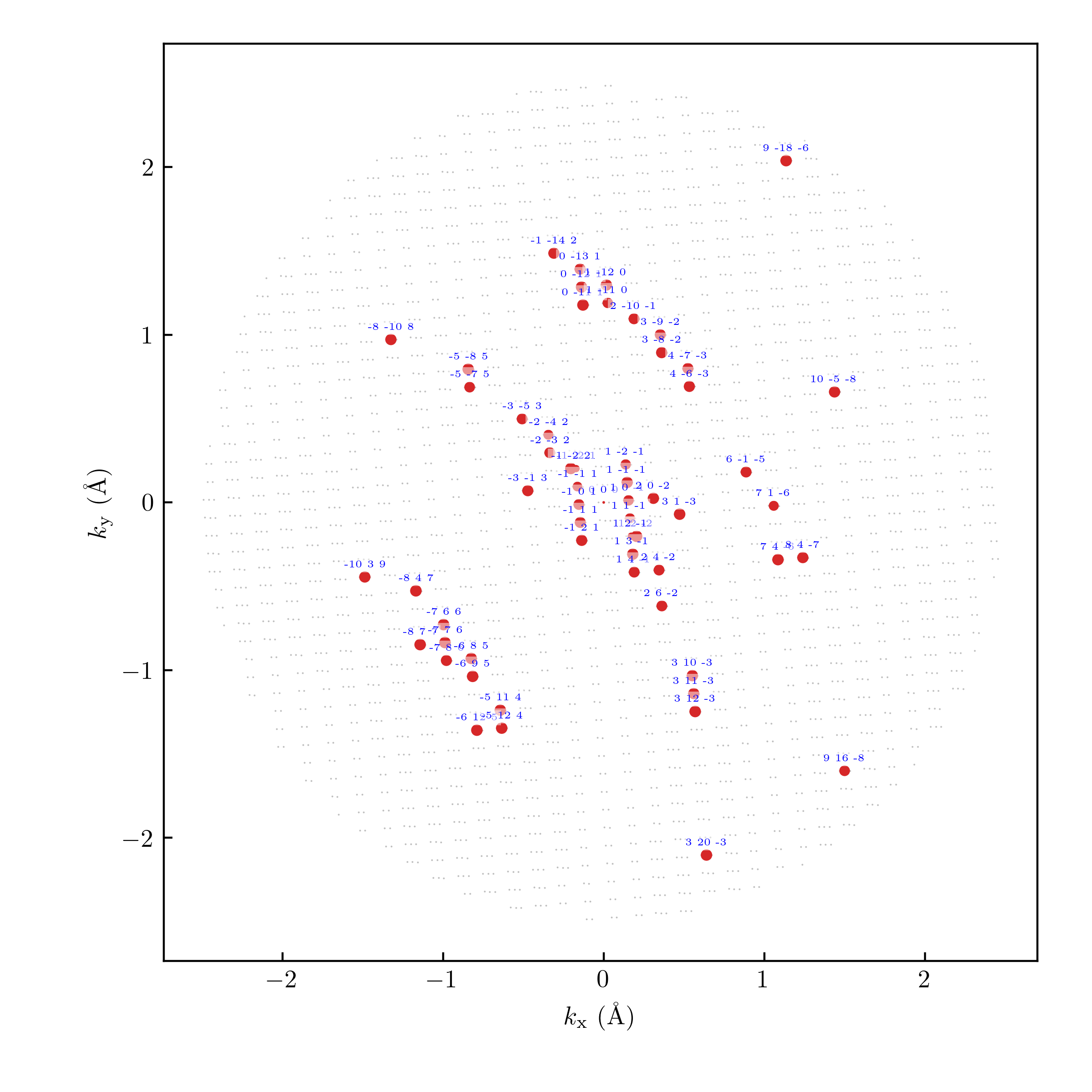
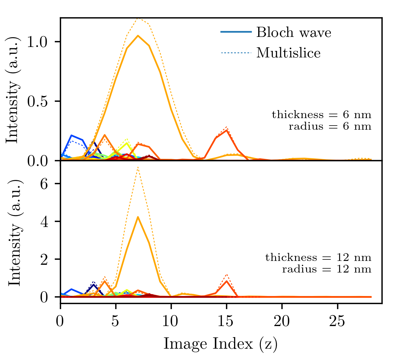
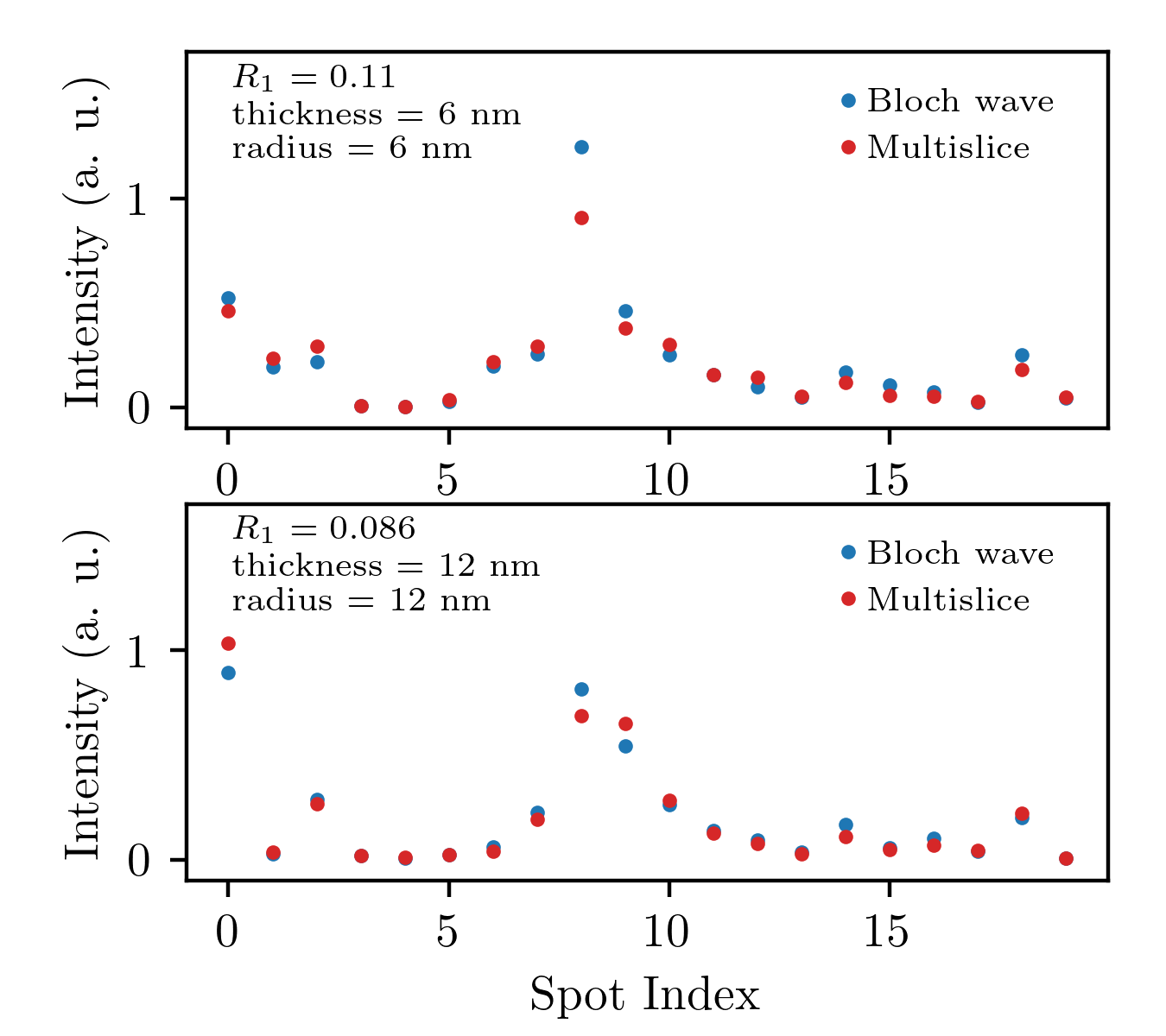
Fig. 4: Same diffraction image as Fig. 3, but now computed using Bloch waves. The red dots mark the high-intensity spots, while the other spots are shown in grey.
Fig. 5: The rocking curves for a group of spots marked in Fig. 4, computed using Bloch wave vs. Multislice (both obtained with abTEM). The upper panel is for a 6 nm thick sample, while the lower panel is for a 12 nm thick sample.
Fig. 6: Spot intensities obtained by integration of rocking curves shown in Fig. 5. The spots are scaled in order to minimize the \(R_1\) factor.
Using a single rotational scan as a basis for comparison, we compute rocking curves with both the Bloch wave and Multislice methods (Fig. 5) and integrate them to obtain spot intensities (Fig. 6). In general, both methods yield similar results, but there remains a small mismatch. The mismatch is probably originating from the finite size of the Multislice system in the xy plane (the plane normal to the beam direction). In the first case (upper panels in Fig. 5 and 6), the cylinder had a radius of 6 nm, whereas in the second (lower panels in Fig. 5 and 6), the radius was 12 nm. The Bloch wave system is considered to be infinite in the xy plane.
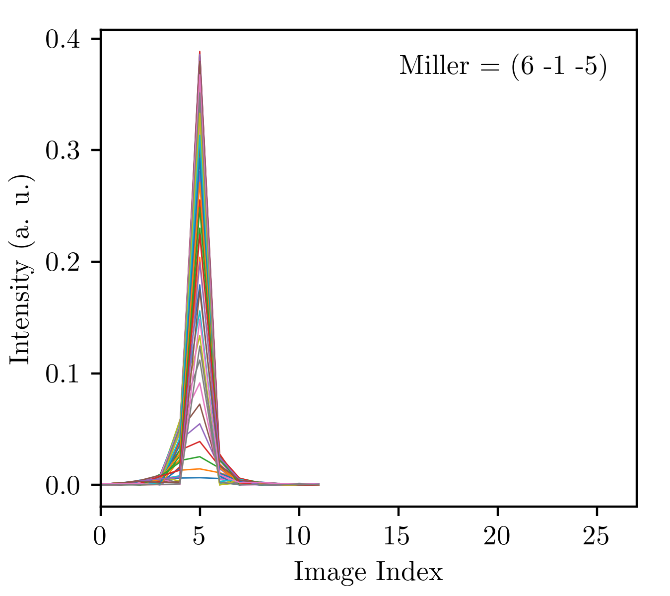
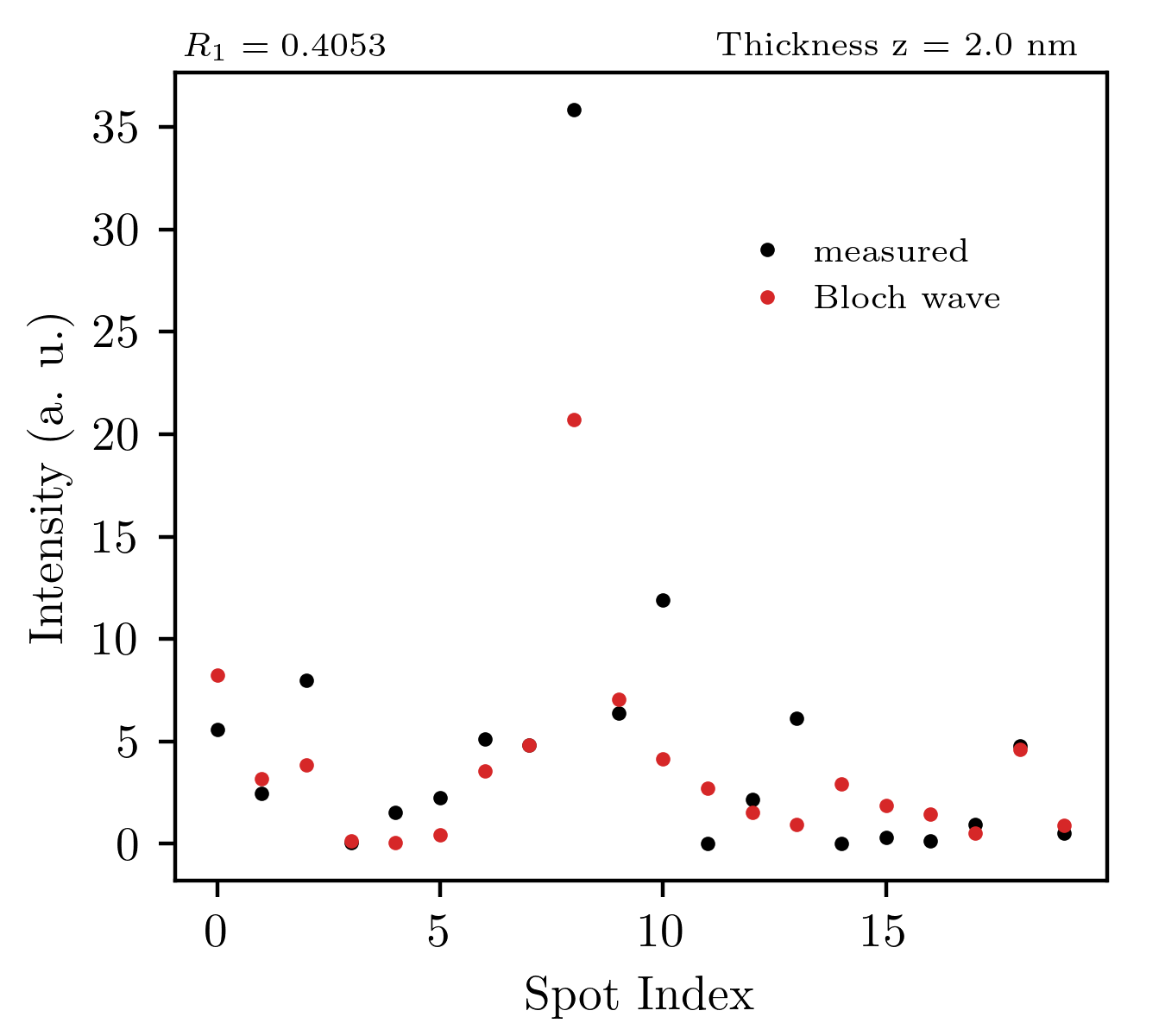
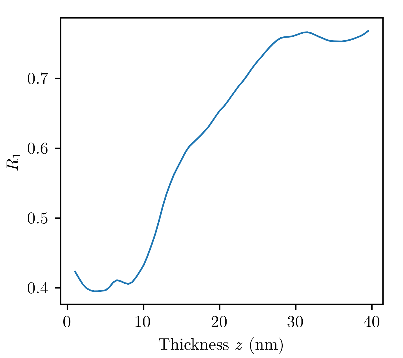
Fig. 7: A rocking curve of a single spot for different crystal thicknesses (obtained using the Bloch wave method). The thickness varies from 1 nm to 40 nm with 0.5 nm step. Higher curves correspond to thicker crystals.
Fig. 8: A comparison of computed (Bloch wave) spot intensities vs. measured for one fixed thickness (Paracetamol data). We used the same spots as in Figs. 4-6.
Fig. 9: The change of R1 factor between the computed (Bloch wave) and measured spot intensities as a function of simulated sample thickness. We picked the same spots as in Figs. 4-6, and Fig. 8.
Next, we can compare the simulation with the experiment. The advantage of the Bloch wave method over Multislice (at least for our system and for thicknesses below 100 nm) is that the calculation can be performed relatively quickly. This allows for scanning different thicknesses and find most probable to produce the observed spots. Fig. 7 shows rocking curves of a single spot for different thicknesses (the higher curves correspond to a thicker sample). The problem with this plot is that it samples the rocking curves only at the image frame orientations. We will need finer rotational sampling in the future.
Fig. 8 compares the Bloch wave results with the measured intensities for a specific thickness. The discrepancy can likely be further reduced by increasing the angular sampling resolution when computing the rocking curves (see the previous paragraph). Fig. 9 shows the $R_1$ factor between the Bloch wave results and the observed intensities as a function of a varying sample thickness. It is clear that there is a thickness range where the computed \(R_1\) factor is minimal, suggesting a possible crystal size.
Discussion
Investigate further the differences between the Bloch wave and the Multislice. Do we get a better match if we increase the size in the xy plane for the Multislice? Check how results converge for different slicing thicknesses in Multislice and for different numbers of beams in Bloch wave (setting different \(k_{\rm max}\)).
When computing the rocking curves, use angular subsampling to obtain smoother results.