05 Feb 2026
- Attendees:
Petrovic, D. McDonagh, D. Waterman, E. Krissinel
Results
The problem we encountered last week was that most spots had a very large intensity range (after scaling all datasets). The question was, is there any parameter that correlates with the spread (for example, an excitation error)? The goal was to pick a single spot and check how its intensity across multiple datasets correlates with its environment or orientation. Figures 1, 2, and 3 show just that (a correlation with the excitation error), for three randomly selected spots. Data with \(I/\sigma < 2\) are grayed out because they might not be very accurate. Spot intensities are scaled between zero and one based on the 97% percentile intensity (to avoid outlier bad spots with unrealistically high intensities).
Figure 4 shows the same plot as Figures. 1-3, but now aggregated for a few spots. In general, we cannot say that there is a correlation between high-intensity spots and zero excitation error. We see that low-intensity spots are noisier, which is expected.
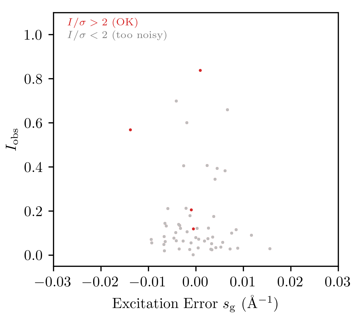
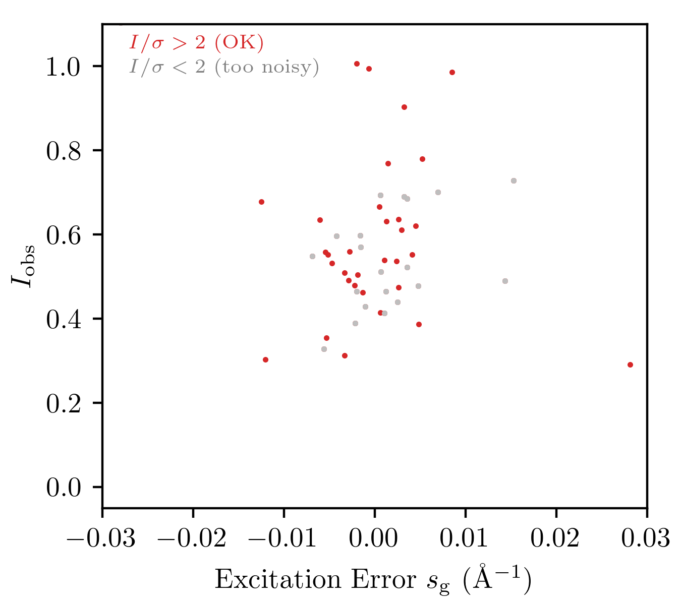
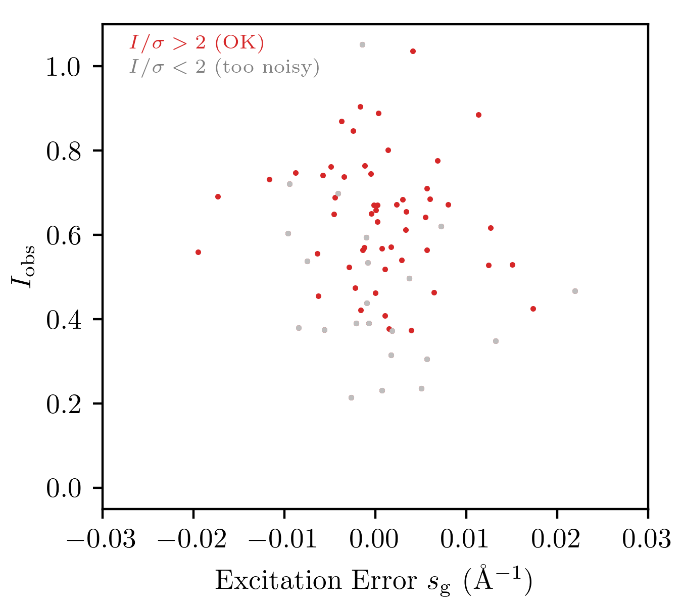
Fig. 1: Spot intensity vs. its excitation error for a single spot (-4, -1, -9). Each point is extracted from a different Paracetamol dataset.
Fig. 2: Same as Fig. 1, but now for spot (-4, -3, -6).
Fig. 3: Same as Fig. 1, but now for spot (-3, 1, -9).
Besides the excitation error, we tried many different quantities that might describe the spot environment on a single image (number of nearest neighbors in the reciprocal space, average weighted neighbor intensity, total number of spots in the image, etc). However, none of them showed any strong correlation with the intensity. For example, in Figs. 5 and 6, we show the results for the number of 3-beam neighbors. Here, for every image where a specific dot \(g = (H,\ K,\ L)\) appears, we counted all the other spot pairs \(g’\) and \(g’’\) that satisfy the condition \(g’ + g’’ = g\). Again, there is no strong correlation with the intensity.
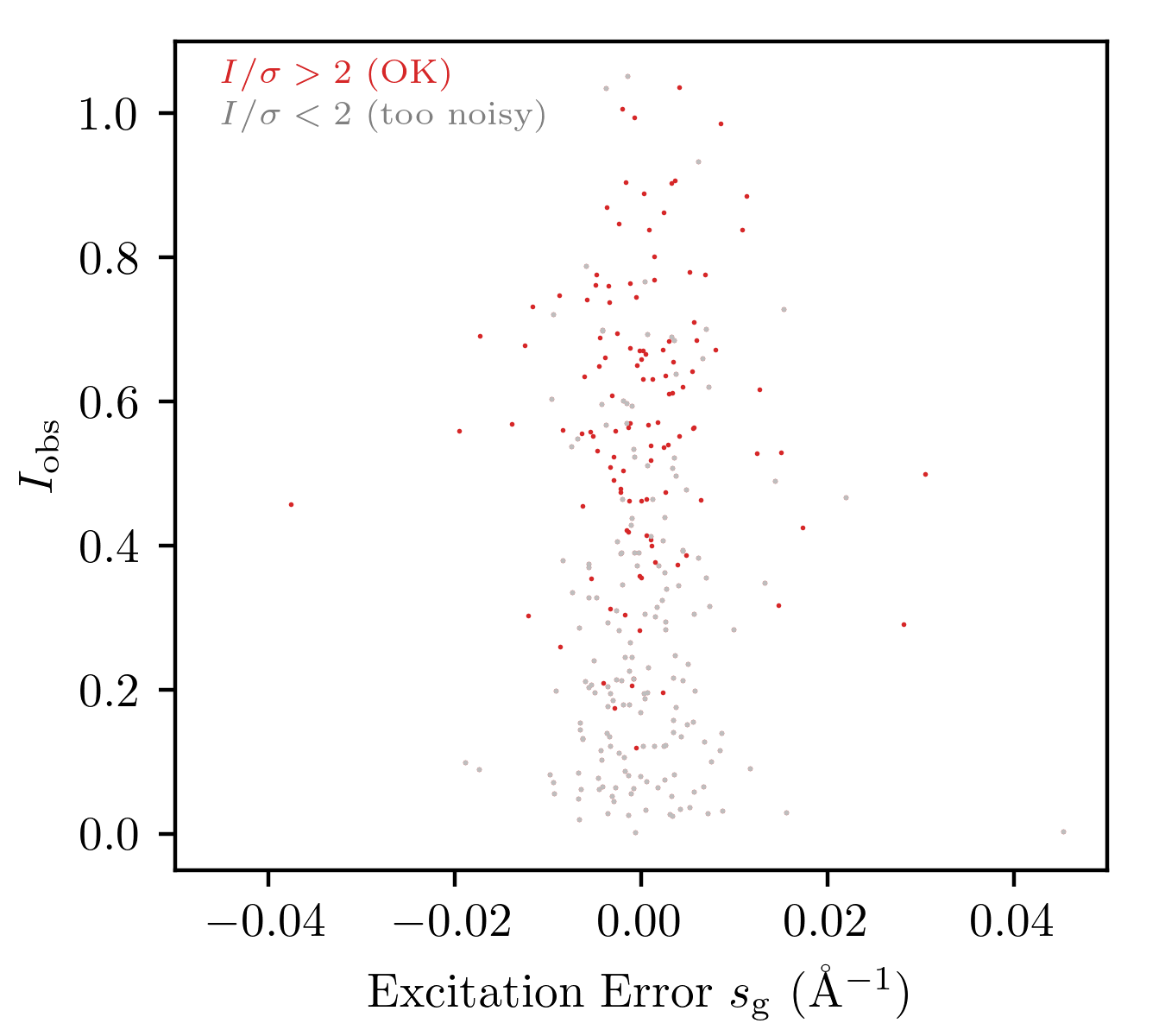
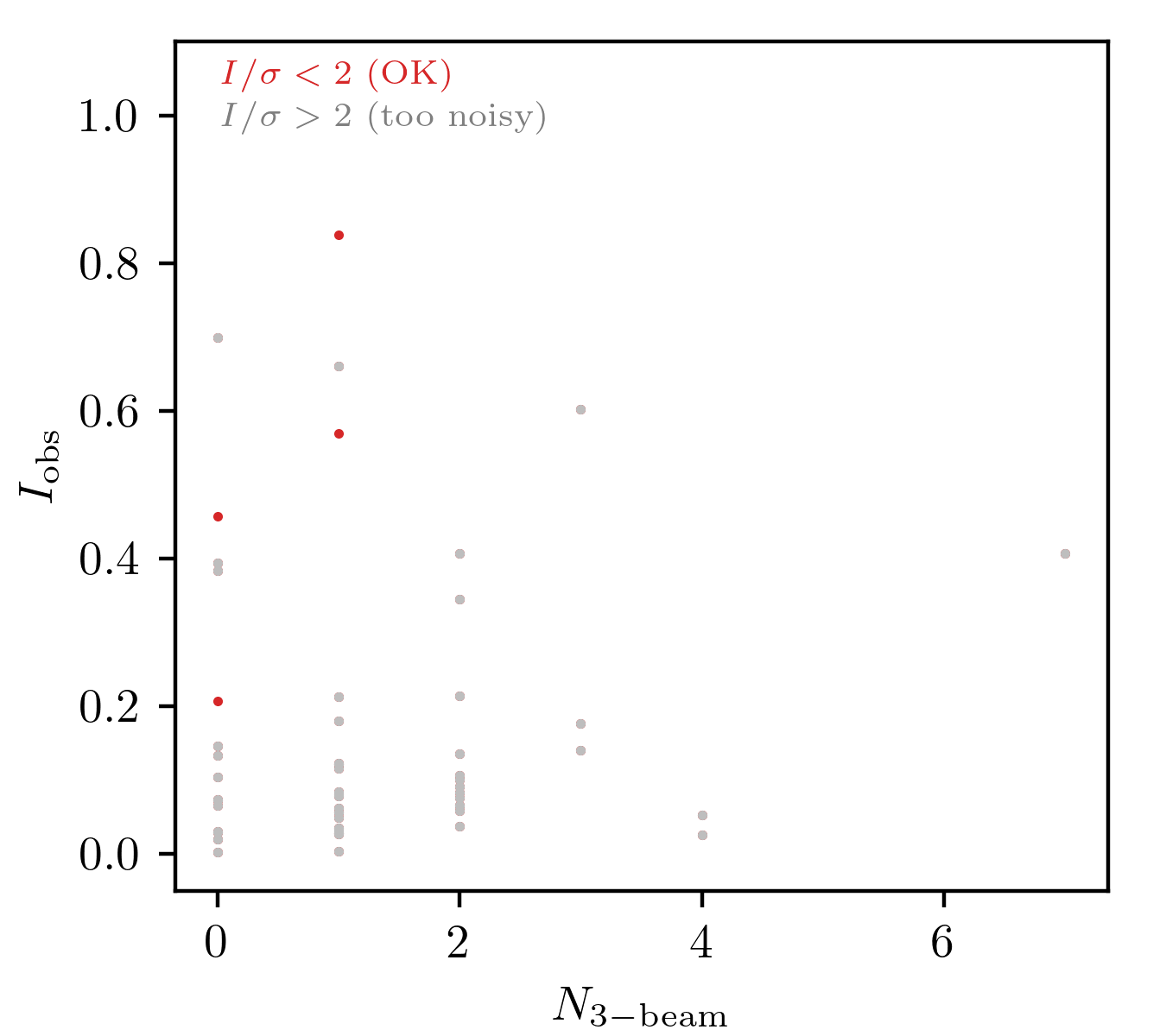
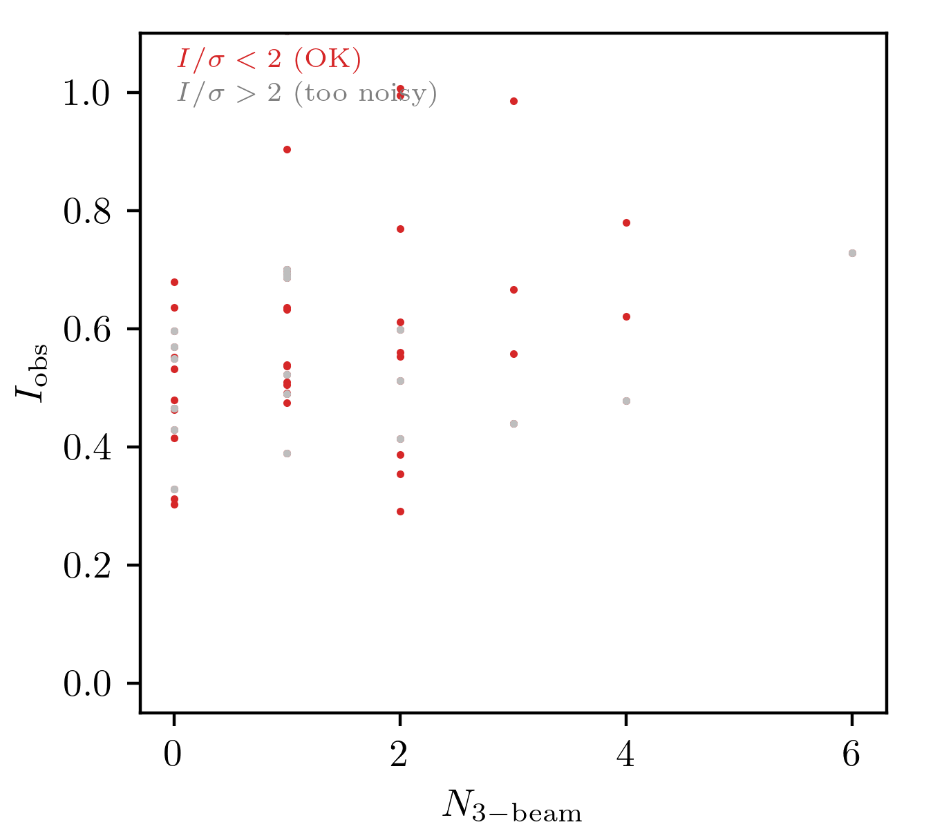
Fig. 4: Same as Figs. 1-3, but now showing aggregate for several spots.
Fig. 5: Number of spots that satisfy the 3-beam condition for the spot (-4, -1, -9). Each point shows the result for a single Paracetamol dataset.
Fig. 6: Same as Fig. 5, but now for spot (-4, -3, -6).
Discussion
All the previous graphs lack the value of \(I_{\rm cal}\) for the solved structure, so it is impossible to say anything about the intensity distribution (which points are above \(I_{\rm cal}\), which are below?).
It is not clear whether the spread in intensity is a consequence of a physical effect, a noise in measurement, or a processing error. We can determine that by processing other datasets (X-ray and electron). If the effect is physical, it can be determined using Bloch-wave or multislice simulations. If the measured data is too noisy, the simulation results can be used for training.
Find datasets with similar orientations (same spot appearing on similar images), and compare the intensities. Might tell us how the environment affects the spot (i.e., is the relative intensity the same or not). One thing this might not account for is thickness. We could have the same orientation but different thicknesses, and therefore get different results.